|
|
1 year ago | |
|---|---|---|
| .. | ||
| audit | 1 year ago | |
| README.md | 1 year ago | |
| w3_day1_neural_network.png | 1 year ago | |
| w3_day1_neuron.png | 1 year ago | |
README.md
Neural Networks
Last week you learnt about some Machine Learning algorithms as Random Forest or Gradient Boosting. Neural Networks are another type of Machine Learning algorithms that are intensively used because of their efficiency. Neural networks are a set of algorithms, modeled loosely after the human brain, that are designed to recognize patterns. They interpret sensory data through a kind of machine perception, labeling or clustering raw input. The patterns they recognize are numerical, contained in vectors, into which all real-world data, be it images, sound, text or time series, must be translated. Different types of neural networks exist and are specific to some use-cases. For example CNN for images, RNN or LSTMs for time-series or text, etc ...
Today we will focus on Artificial Neural Networks. The goal is to understand how do the neural networks work, train them on data and understand the challenges of training a neural network. The ressources below expalin very well the mecanisms behind neural networks, step by step.
However the exercices won't cover architectures as RNN, LSTM - used on sequences as time series or text, CNN - used a lot on images processing. One of the projects will require to know how to use the special architectures. To do so, I suggest that you go through this lesson: https://fr.coursera.org/specializations/deep-learning.
Exercises of the day
- Exercise 0: Environment and libraries
- Exercise 1: The neuron
- Exercise 2: Neural network
- Exercise 3: Log loss
- Exercise 4: Forward propagation
- Exercise 5: Regression
Virtual Environment
- Python 3.x
- NumPy
- Jupyter or JupyterLab
Version of NumPy I used to do the exercises: 1.18.1. I suggest to use the most recent one.
Resources
Exercise 0: Environment and libraries
The goal of this exercise is to set up the Python work environment with the required libraries.
Note: For each quest, your first exercice will be to set up the virtual environment with the required libraries.
I recommend to use:
- the last stable versions of Python.
- the virtual environment you're the most confortable with.
virtualenvandcondaare the most used in Data Science. - one of the most recents versions of the libraries required
- Create a virtual environment with a version of Python >=
3.8, with the following libraries:numpyandjupyter.
Exercise 1: The neuron
The goal of this exercise is to understand the role of a neuron and to implement a neuron.
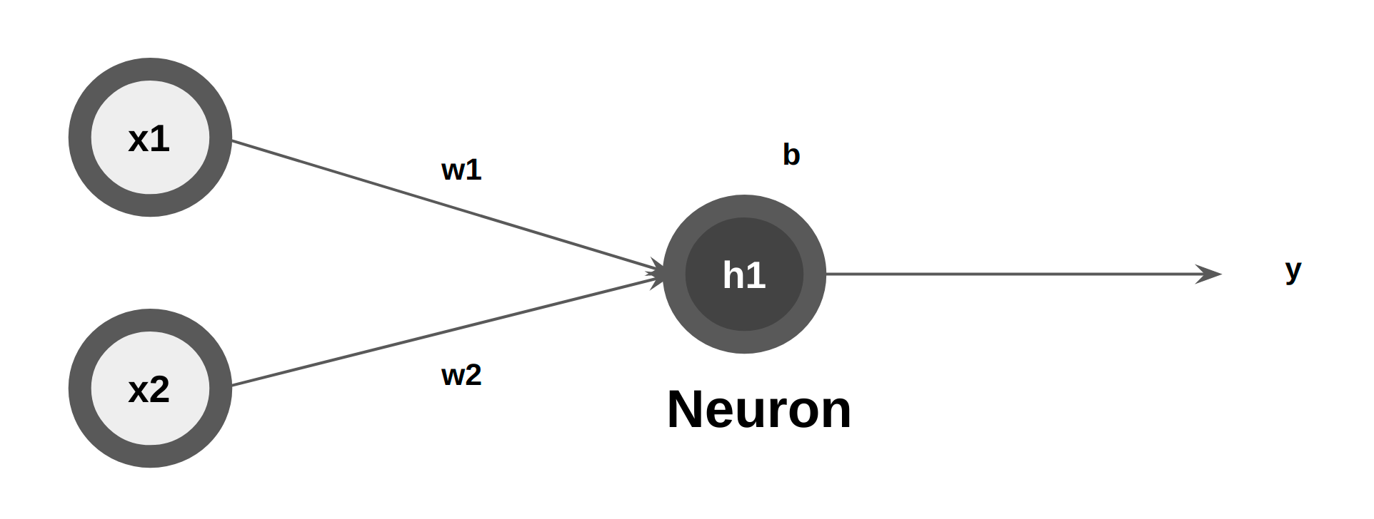
An artificial neuron, the basic unit of the neural network, (also referred to as a perceptron) is a mathematical function. It takes one or more inputs that are multiplied by values called “weights” and added together. This value is then passed to a non-linear function, known as an activation function, to become the neuron’s output.
As desbribed in the article, a neuron takes inputs, does some math with them, and produces one output.
Let us assume there are 2 inputs. Here are the three steps involved in the neuron:
-
Each input is multiplied by a weight
- x1 -> x1 * w1
- x2 -> x2 * w2
-
The weighted inputs are added together with a biais b
- (x1 _ w1) + (x2 _ w2) + b
-
The sum is passed through an activation function
-
y = f((x1 _ w1) + (x2 _ w2) + b)
-
The activation function is a function you know from W2DAY2 (Logistic Regression): the sigmoid
-
Example:
x1 = 2 , x2 = 3 , w1 = 0, w2= 1, b = 4
- Step 1: Multiply by a weight
- x1 -> 2 * 0 = 0
- x2 -> 3 * 1 = 3
- Step 2: Add weigthed inputs and bias
- 0 + 3 + 4 = 7
- Step 3: Activation function
- y = f(7) = 0.999
-
Implement a the function feedforward of the class
Neuronthat takes as input the inputs (x1, x2) and that uses the attributes: the weights and the biais to return y:class Neuron: def __init__(self, weight1, weight2, bias): self.weights_1 = weight1 self.weights_2 = weight2 self.bias = bias def feedforward(cls, x1, x2): #TODO return y
Note: if you are confortable with matrix multiplication, feel free to vectorize the operations as done in the article.
https://victorzhou.com/blog/intro-to-neural-networks/
Exerice 2: Neural network
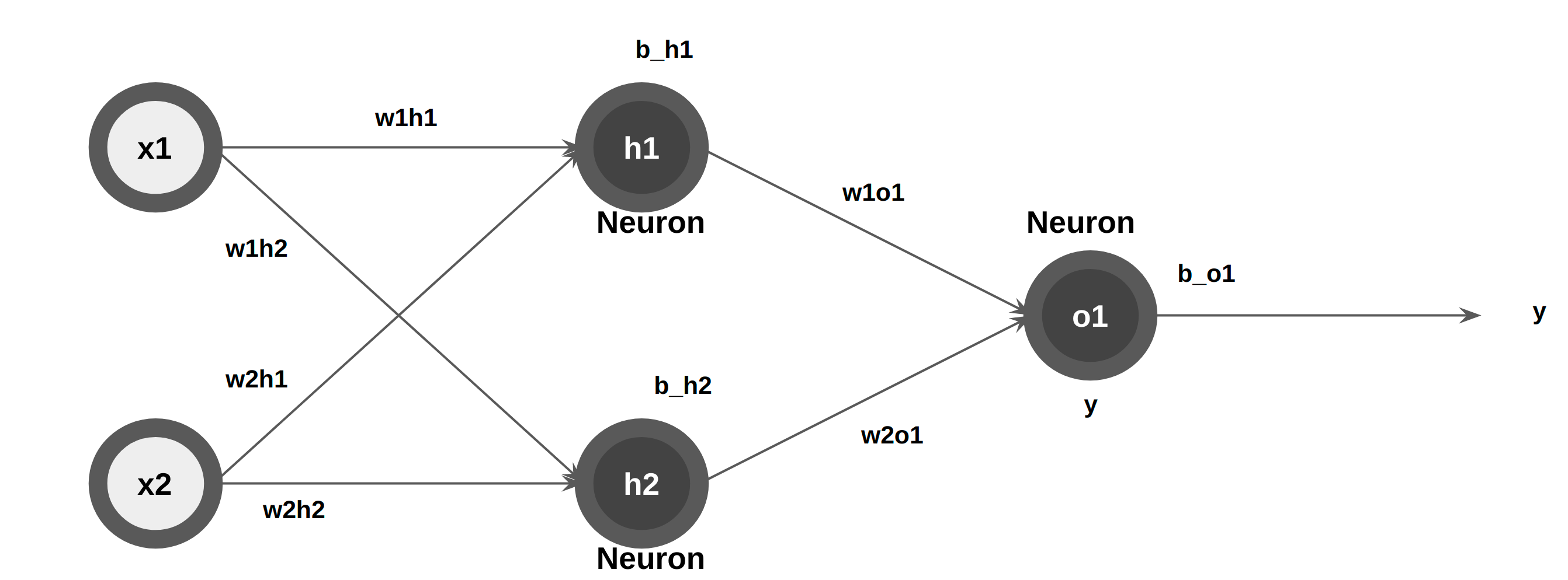
The goal of this exercise is to understand how to combine three neurons to form a neural network. A neural newtwork is nothing else than neurons connected together. As shown in the figure the neural network is composed of layers:
- Input layer: it only represents input data. It doesn't contain neurons.
- Output layer: it represents the last layer. It contains a neuron (in some cases more than 1).
- Hidden layer: any layer between the input (first) layer and output (last) layer. Many hidden layers can be stacked. When there are many hidden layers, the neural networks is deep.
Notice that the neuron o1 in the output layer takes as input the output of the neurons h1 and h2 in the hidden layer.
In exercise 1, you implemented this neuron.

Now, we add two more neurons:
- h2, the second neuron of the hidden layer
- o1, the neuron of the output layer
-
Implement the function
feedforwardof the classOurNeuralNetworkthat takes as input the input data and returns the output y. Return the output for these neurons:neuron_h1 = Neuron(1,2,-1) neuron_h2 = Neuron(0.5,1,0) neuron_o1 = Neuron(2,0,1)class OurNeuralNetwork: def __init__(self, neuron_h1, neuron_h2, neuron_o1): self.h1 = neuron_h1 self.h2 = neuron_h2 self.o1 = neuron_o1 def feedforward(self, x1, x2): # The inputs for o1 are the outputs from h1 and h2 # TODO return y
Exercise 3: Log loss
The goal of this exercise is to implement the Log loss function. As mentioned last week, this function is used in classification as a loss function. It means that the better the classifier is, the smaller the loss function is. W2D1, you implemented the gradient descent on the MSE loss to update the weights of the linear regression. Similarly, the minimization of the Log loss leads to finding optimal weights.
Log loss: - 1/n * Sum[(y_true*log(y_pred) + (1-y_true)*log(1-y_pred))]
-
Create a function
log_loss_customand compute the loss for the data below:``` y_true = np.array([0,1,1,0,1]) y_pred = np.array([0.1,0.8,0.6, 0.5, 0.3]) ``` Check that `log_loss` from `sklearn.metrics` returns the same resulthttps://scikit-learn.org/stable/modules/generated/sklearn.metrics.log_loss.html
Exercise 4: Forward propagation
The goal of this exerice is to compute the log loss on the output of the forward propagation. The data used is the tiny data set below.
| name | math | chemistry | exam_success |
|---|---|---|---|
| Bob | 12 | 15 | 1 |
| Eli | 10 | 9 | 0 |
| Tom | 18 | 18 | 1 |
| Ryan | 13 | 14 | 1 |
The goal if the network is to predict the success at the exam given math and chemistry grades. The inputs are math and chemistry and the target is exam_sucess.
-
Compute and return the output of the neural network for each of the students. Here are the weights and biases of the neural network:
neuron_h1 = Neuron(0.05, 0.001, 0) neuron_h2 = Neuron(0.02, 0.003, 0) neuron_o1 = Neuron(2,0,0) -
Compute the logloss for the data given the output of the neural network with the 4 students.
Exercise 5: Regression
The goal of this exercise is to learn to adapt the output layer to regression. As a reminder, one of reasons for which the sigmoid is used in classification is because it contracts the output between 0 and 1 which is the expected output range for a probability (W2D2: Logistic regression). However, the output of the regression is not a probability.
In order to perform a regression using a neural network, the activation function of the neuron on the output layer has to be modified to identity function. In mathematics, the identity function is: f(x) = x. In other words it means that it returns the input as so. The three steps become:
- Each input is multiplied by a weight
- x1 -> x1 * w1
- x2 -> x2 * w2
- The weighted inputs are added together with a biais b
- (x1 _ w1) + (x2 _ w2) + b
- The sum is passed through an activation function
- y = f((x1 _ w1) + (x2 _ w2) + b)
- The activation function is the identity
- y = (x1 _ w1) + (x2 _ w2) + b
All other neurons' activation function doesn't change.
-
Adapt the neuron class implemented in exercise 1. It now takes as a parameter
regressionwhich is boolean. When its value isTrue,feedforwardshould use the identity function as activation function instead of the sigmoid function.class Neuron: def __init__(self, weight1, weight2, bias, regression): self.weights_1 = weight1 self.weights_2 = weight2 self.bias = bias #TODO def feedforward(self, x1, x2): #TODO return y-
Compute the output for:
neuron = Neuron(0,1,4, True)
neuron.feedforward(2,3)
-
-
Now, the goal of the network is to predict the physics' grade at the exam given math and chemistry grades. The inputs are
mathandchemistryand the target isphysics.
| name | math | chemistry | physics |
|---|---|---|---|
| Bob | 12 | 15 | 16 |
| Eli | 10 | 9 | 10 |
| Tom | 18 | 18 | 19 |
| Ryan | 13 | 14 | 16 |
Compute and return the output of the neural network for each of the students. Here are the weights and biases of the neural network:
    #replace regression by the right value
    neuron_h1 = Neuron(0.05, 0.001, 0, regression)
    neuron_h2 = Neuron(0.002, 0.003, 0, regression)
    neuron_o1 = Neuron(2,7,10, regression)
- Compute the MSE for the 4 students.
